Copyright (c) 2023 Massachusetts Institute of Technology

SPDX-License-Identifier: MIT

Concept Probing Using Sparse Perturbations

This notebook demonstrates how the gradient_ascent function from the previous tutorial can be repurposed with a different optimizer (L1qFrankWolfe) to execute a task called concept probing. This method of concept probing was first reported in the paper Controllably Sparse Perturbations of Robust Classifiers for Explaining Predictions and Probing Learned Concepts.

If you haven’t already, follow the steps at the beginning of the previous tutorial to install the rAI-toolbox and create a Jupyter notebook called ImageNet-Concept-Probing.ipynb. You can then follow along with this tutorial by copying, pasting, and running the code blocks below in the cells of your notebook.

Boilerplate setup

from functools import partial

import torch
import matplotlib.pyplot as plt

from rai_toolbox.optim import L1qFrankWolfe
from rai_toolbox.perturbations import gradient_ascent

from rai_experiments.utils.imagenet_labels import IMAGENET_LABELS

# CPU or GPU
device = "cuda:0" if torch.cuda.is_available() else "cpu"
print(device)

cuda:0

Load pre-trained ImageNet models

The pre-trained models used in this example are simplified data structures of the pre-trained models available via Madrylab’s robustness library README for the ImageNet dataset, and include:

• mitll_imagenet_l2_3_0.pt: ResNet-50 model trained with perturbations generated via PGD using the \(L^2\)-norm with \(\epsilon=3.0\)

• imagenet_nat.pt: ResNet-50 model trained using standard training, i.e., \(\epsilon=0\)

rai_experiments.models.pretrained.load_model will automatically download and cache pre-trained weights for these models.

from rai_experiments.models.pretrained import load_model

# Load the robust model
model_robust = load_model("mitll_imagenet_l2_3_0.pt")
model_robust.eval();

# Load the standard model
model_standard = load_model("imagenet_nat.pt")
model_standard.eval();

Concept probing

We will now demonstrate how the optimizer input to gradient_ascent can be switched out to complete a different task, called Concept Probing. Now instead of starting with a real image from the test set and optimizing its perturbation away from its true class as we did in the previous tutorial, in this example, we’ll be starting with a random noise image and optimizing its perturbation towards a class of interest, in an attempt to visualize what the model has learned for that class.

Following the approach proposed by the authors of this paper, we utilize the \(L^{1-q}\) Frank-Wolfe optimizer to solve for sparse perturbations that are more interpretable by humans.

We will use functools.partial to set default values for gradient_ascent, so that they can be used consistently across our two models. Note that AdditivePerturbation is the default perturbation_model for gradient_ascent, so we don’t need to define it explicitly.

# Define solver for concept probing example:
solver_L1FW = partial(
    gradient_ascent,
    optimizer=L1qFrankWolfe,
    # optimizer options
    lr=1.0,
    epsilon=7760,
    q=0.975,
    dq=0.05,
    # solver options
    steps=45,
    targeted=True,
    use_best=False
)

Define three concepts to be probed (e.g., target classes), a random noise image to start with, and a function for probing those three concepts for a given model:

# Concepts to be probed
target_classes = [75, 17, 965]

# Random noise image
init_noise = torch.randn([1, 3, 224, 224])
init_noise = init_noise - init_noise.min()
init_noise = init_noise / init_noise.max()

# Function for probing concepts
def probe_concepts(x, target_classes, solver, model):
    _, ax = plt.subplots(2,3,figsize=(10,5))
    for i in range(3):
        # optimize loss towards target class
        target = torch.tensor([target_classes[i]])

        # run solver
        x_concept, _ = solver(
            model=model.to(device),
            data=x.to(device),
            target=target.to(device),
        )

        # plot
        ax[0, i].imshow(x[0].permute(1,2,0))
        ax[0, i].axis("off")
        ax[1, i].set_title(IMAGENET_LABELS[target_classes[i]].partition(",")[0])
        ax[1, i].imshow(x_concept[0].detach().cpu().clamp_(0,1).permute(1,2,0))
        ax[1, i].axis("off")

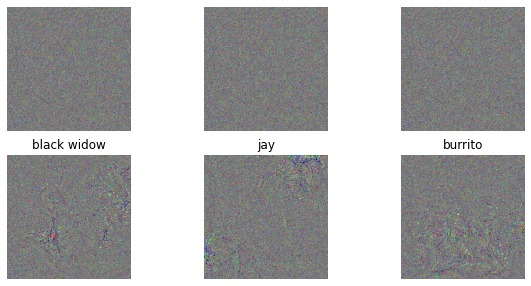
Run for standard and robust models and plot (first row is initial noise image, second row is the probed concept):

# Standard
probe_concepts(init_noise, target_classes, solver_L1FW, model_standard)

# Robust
probe_concepts(init_noise, target_classes, solver_L1FW, model_robust)

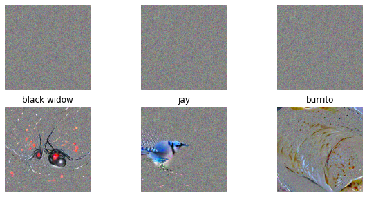
Note that the concepts from the robust model are much more pronounced and look like the target class to the human eye.